Radial Basis Function Neural Networks Theory And Applications

As we have progressed through the technological world, biological functions are being mimicked into the technological arena. One such venture is the artificial intelligence area, the basis of which is the artificial neural network. This is the mimicry of biological neural structure, which memorizes and learns, building intelligence for a living being. The same concept is applied to systems such that individual data patterns are identified, memorized, and eventually learned for system predictions. The background of such system functioning is the algorithms, which create an artificial neural network, that gets better over time; thus behaving like an individual intelligent programmed system

One such advanced and widely used neural network system is the “radial basis function network”(RBF). This is a single direction, multi-layer neural network with three functional layers. The advantage of this type of network is faster learning of the systems and shorter training periods for system evaluations. These neural networks find their place in prediction models especially related to defect/anomaly systems; found in finance, shares, and economic frauds.

Layers of Network

1. Input layer

The input layer in a Radial Basis Function (RBF) neural network is responsible for receiving and processing the initial data fed into the system. This layer consists of multiple nodes, each representing a different input feature or data point. The design of this layer is crucial because the number of input nodes determines the dimensions of the input data the network can handle.

For instance, if you are working with a dataset containing five features, the input layer will have five nodes, each corresponding to one of those features. The quality and relevance of the data inputs are paramount, as they directly impact the network’s ability to learn and make accurate predictions. Essentially, the input layer serves as the foundation for the subsequent processing and learning stages in the RBF network, where each input node passes the data onto the next layer for further transformation and analysis.

2. Hidden layer

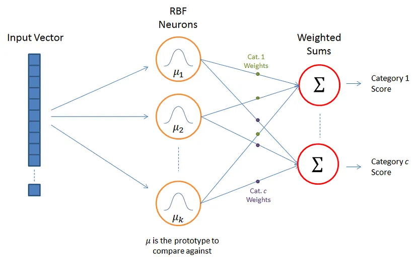
This refers to a number of neurons, each composed of a radial basis function. Each of this function consists of a central portion and width (non-linear) parameter. Once the center and width are mapped, the input vectors are mapped to each of these radial functions, the collective interactions of which give us the output. The input interactions with the hidden layers are calculated as a function, which can be either, Gaussian, thin-plate Spiline or Cauchy calculations. The most commonly used is the Gaussian function. Further, the program is optimized using various algorithms. The layers in this neural network can be described using the figure below:

3. Output layer

This is essentially a set of nodes, each belonging to the group that is being classified. They are individually scored to the associated group, in relation to the input parameters. The distance between the input and the output vectors are usually taken as then Euclidean distance. These scores are then computed considering each of the RBF functions.

Every output node will have its own weight sets as each output node will compute scores differently. This ensures the RBF neurons get the positive weight received by the output node belonging to its category, and a negative weight to the others. These output sets are then normalized and trained using gradient descent.

Training the Output values

The training process are determined by several parameters including

1. Number of neurons in the hidden layer

2. Coordinates of the centre of each of those layers

3. Radius (spread)/width of each RBF function in each dimension.

4. Weights applied to the outputs in each case considered.

The networks are typically trained using the k-means clustering, when unsupervised; or a simple linear model with co-efficient. There is also a third optional back-propagation step that could be incorporated, where the parameters are weighed to their effect over the output and fed back into the program.

Applications of Radial Basis Function Neural Network

RBF networks are quick learners and training these algorithms is also very quick and efficient. Owing to these properties, they are widely used in pattern recognitions software’s, financial transaction monitoring, fraud monitoring software, time series prediction. Each of the parameters of this network can be individually controlled and modified as need be. The RBF networks are also using in studying EEG functions and health monitors. Other applications include fault diagnosis in access networks, recognition if wireless standards, antenna array signal processing, channel equalization among others. The RBF neural networks also have hardware applications. They are used in building analogue circuits; pulsed very large scale integration (VLSI) RBF network chips (both direct digital and hybrid implementations).

• Having learned the basic principles of this network and its applications, let us now move towards its advantages over other network systems. Some of the most notable ones are:
• The design of the RBF network is simple and easy• It is very flexible and has high tolerance to input noise
• It is easy to train the algorithms in RBF networks rather than multi-layer perceptrons.
• Designing and ordering parameters is easier in RBF
• The program learns faster online compared to other networks
• It has efficient generalization capability and gives better results in fuzzy input environments
• The biggest advantage of the RBF neural network is that it has universal approximation and regulation capabilities, due to which it can have vast applications.

Let us now move towards tools that implement RBF networks

KEEL: Knowledge Extraction based on Evolutionary Learning (KEEL), an open source (GPLv3) Java tool which empowers the user to assess the behaviour of evolutionary learning and soft computing for different kinds of DM problems like regression, classification, clustering, pattern study etc.

WEKA: This is a Guassian RBF network implemented in Java. This uses k-means clustering algorithm and learns by regression models.

MATLAB: This works by implementing two functions, namely, newrb — that add neurons to the hidden layer of the RBF network and that quickly designs radial basis functions with zero errors. In this model, the larger the spread of hidden layers, the smoother the function approximation.

DTREG: This is open source software for predictive modelling and forecasting.

NETLAB: This is a toolbox to provide the necessary simulation of theoretically well founded neural network algorithms to be used in research, teaching, and application development.

Although many great accomplishments can be done using this technology, it is far from being a digital copy of the human brain. Its trial and implementation in every possible area of life and observations for further training is the key to evolve these programs.

Several data sets have successfully been used to automate accurate algorithms. Some of them include data sets for Iris (99.36% accuracy), wine (97.9%), glass (92.7%), new thyroid (96.59%), diabetes (78.02%), hepatitis (90.33%), heart (90.33%), liver (74.26%), breast cancer( 99.43%), lung cancer (67.78%), satellite images (90.35%). Developing more such parameters for unsupervised learning is believed to accelerate the implementation of artificial intelligence in daily lives.

FAQs about Radial Basis Function Neural Networks